Introduction
LitSplot, which can be read as “Let’s Plot” and otherwise pronounced as “LIghT’S-PLOTs,” is a tool purposed for the post processing capabilities of the “EXYE” flagship programme.
Post processing of a finite element data refers to the way numerical results are interpreted and presented, in a useful way for user convenience and industry applications. Compliance to standards, checks and filters, transformations, logging, and value-added operations are primarily included in the software package, or they come as separate tools dedicated to post processing. LitSplot falls in the latter category.
Finite Element Method
Finite Element Method is a method of numerically solving complex physical problems. This method deals with converting the physical definitions of the problem viz, shape, size, boundary, loads, inputs, frames of reference, and observation into simpler numerical meshes. These parameters are maintained and modelled with utmost accuracy to retain the actual or near-actual complexities. The set of equations governing the phenomenon are further solved at each element of the mesh, assuming the behaviour of the parameter to remain invariant over the finitely small range contrary to the macroscopic variation over the entire finite volume in consideration. These solutions are then aggregated or compounded over the entire domain of analysis. The results obtained here are hence approximate in nature.
FEA traces its origin as a method of stress analysis in the design of aircraft wings and further complex structures. Today, not only structural, and mechanical domains have found its applications but also fluid dynamics and kinematics. With improved computing power and expanding knowledge of concept, equations, and skills in development of algorithms the method can be used for complex problems like heat transfer, magnetic and electric fields, and fluxes
Given the flexibility in the method, it can be used similarly in both static and dynamic problems.
Defining the Problem
The FEM problem involves identifying the problem, the target solution and subsequently formulating a way to achieve the same. Understanding the input and breaking it into steps of finite size to formulate a relevant grid is the first and the foremost step.
Creation and refinement of the grid, called as the mesh, is followed by identifying the relevant set of rules, regulations, and governing equations to explain the phenomenon under consideration.
Finally, the results are returned in the form of arrays of solutions over the entire domain defined over the mesh. These results can be integrated, summarized, or visualized as per the need of the problem.
Input
Current version of the tool takes the output from general purpose optical simulation software. The inputs are in the form of photometric maps of intensity from a given light source for a targeted function.
The inputs to the post processing tool are derived from the tools which are already utilizing FEM to formulate the photometric maps. Hence, the inputs too have a uniform step increment and discrete value defined at each node of the element mesh.
Visualization
The data obtained from various tools have different domains and techniques of projection. Visualization requires the users to focus on the angular gradient of concern and thereby eliminate the coarse environment from the finer control surface.
Furthermore, these control surfaces are defined by various regulatory organizations (SAE, UNECE, IES etc.) from various parts of the globe. These organizations also lay certain thumb rules to be complied with for legalization and safety regulation of lighting solutions. These regulations and compliance also come as an added factor to report the visualization of results for the purpose of consumption
Projection
Given the application of the automotive lighting to see on the road, the projection of the photometric map on the road inevitably becomes a crucial part of the visualization. However, projection is not merely a translation problem but also a transformation scenario making it a full-fledged FEM statement which requires a numerical solution.
The intensity varies in an angular pattern and the road in a spatial gradient. The first step of simplification is to transform the spatial gradient into angular grid by mapping corresponding elements of the spatial mesh to its unique one to one relation in the corresponding angular domain. Since the resolution of the spatial gradient is linear, but the mapping factor varies by a factor of trigonometric tangent, the domain needs to be interpolated for the required mapped values.
Next, the distance between the assumed point emitting the illumination function and the mapped nodes needs to be evaluated and stored in a transformation matrix to apply the inverse square law to convert photometric intensity into illuminance.
Literature Survey
Given the focus and scope of our study is centred around the development of a post processing tool, the primary essence is to understand the type of outputs generated by the solvers in market.
Since the tool is specific to the software domain of lighting and optics applications, various formats of storing optical data (specifically standardised and open source with no commercial association); methodologies and conditions governing visualization and projection; resolution of data becomes crucial aspects of the study.
Goniometry/ Gonio-photometry
A Goniophotometer is a device used to measure light emitted from an object at different angles. The use of goniometers is specific to the functions which are direct sources of light. Due to strict regulations, the spatial distribution of light is of high importance to automobile industry. Hence, the targeted lighting function is assumed to be a point emittance and is accordingly mapped.
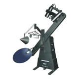
Fig: Goniophotometer
Mercator Projection
Mercator projection is the map we are most familiar with. Developed by a Dutch mathematician Gerhardous Mercator in 1569, this method is used for cartography. The salient features of the maps charted off this method in context to cartography and has been postulated in the following three properties.
The immediate result of these three properties is that the Mercator projection maps rhumb lines on the sphere into straight lines, and vice versa.
Application extended to spherical spread from the assumed point function to a 2-D map eases both visualization and operation on the output post simulation.
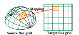
Fig: Mapping to a Projection
IESNA
Illumination Engineers Society of North America (IESNA) is an organization with nearly 50 technical committees comprised of over 1,000 volunteer subject matter experts. The standards established by the society in 1991 serve as the basic governors for goniometric projections based out of essentially 3 types of goniometers and hence 3 different denotations specific to the projection axes and applications.
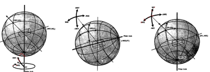
Fig: Type-A, Type-B, and Type-C projections IES
Out of these three categories of IES files documenting the projections – type A and type C are relevant to our goal. They are projections about the first axial flattening about the polar axis and are used for automotive and general-purpose lighting, respectively.
In addition to the concepts and conventions of IESNA, IES file formats storing the metadata and intensity distribution in the form of plain text to simulate the light with the defined architectural layout, were studied and encoded into a process.
Procedure
The photometric data received as the output from the commercial solver is exported to EXR/IES formats which are open source and usable outside the domain of the licenses. This output is converted into intensity arrays and stored into the memory of the computer.
These arrays are further:
Data and Validation
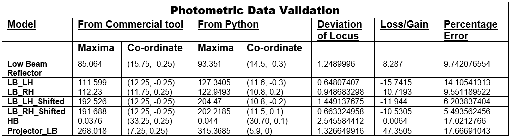
The following data has been recorded for various configurations. The recorded data was processed in the inbuilt post processing tool of the commercial software and the currently developing LitSplot utility. The Validation results were recorded as follows:
Conclusion
The algorithm can cater to the basic post processing visualization needs which enables it to become an appropriate add on to the Lucid Shape outputs.
The data recorded shows illumination patterns like the ones obtained from the Lucid Shape post-processing. The maximum illuminance is the quantitative measure to establish the values projection.
The intensity measured is recorded as the quantitative factor for the translation function of the photometric map to road illumination. The average deviation of 11.39 % ranging between [5.4 to 17.67] %. The qualitative factor is given by the location of maximum brightness on the road. The locus of this maxima conforms the standardizing data set with an average deviation of 1.26m ranging between [0.6 to 2.54] m.
The accuracy factor may be better standardised against experimental data. Also, an internal solver catering the optical phenomenon may add to the accuracy of the data.